navis.plot2d¶

navis.plot2d(x, method='3d', **kwargs)[source]¶

Generate 2D plots of neurons and neuropils.

The main advantage of this is that you can save plot as vector graphics.

Important

This function uses matplotlib which “fakes” 3D as it has only very limited control over layering objects in 3D. Therefore neurites are not necessarily plotted in the right Z order. This becomes especially troublesome when plotting a complex scene with lots of neurons criss-crossing. See the method parameter for details. All methods use orthogonal projection.

Parameters:

x (TreeNeuron | MeshNeuron | NeuronList | Volume | Dotprops | np.ndarray) –
Objects to plot:
- multiple objects can be passed as list (see examples)
- numpy array of shape (n,3) is intepreted as points for scatter plots
method ('2d' | '3d' (default) | '3d_complex') –
Method used to generate plot. Comes in three flavours:
1. ’2d’ uses normal matplotlib. Neurons are plotted on top of one another in the order their are passed to the function. Use the view parameter (below) to set the view (default = xy).
2. ’3d’ uses matplotlib’s 3D axis. Here, matplotlib decide the depth order (zorder) of plotting. Can change perspective either interacively or by code (see examples).
3. ’3d_complex’ same as 3d but each neuron segment is added individually. This allows for more complex zorders to be rendered correctly. Slows down rendering though.
soma (bool, default=True) – Plot soma if one exists. Size of the soma is determined by the neuron’s .soma_radius property which defaults to the “radius” column for TreeNeurons.
connectors (bool, default=True) – Plot connectors.
connectors_only (boolean, default=False) – Plot only connectors, not the neuron.
cn_size (int | float, default = 1) – Size of connectors.
linewidth (int | float, default=.5) – Width of neurites. Also accepts alias lw.
linestyle (str, default='-') – Line style of neurites. Also accepts alias ls.
autoscale (bool, default=True) – If True, will scale the axes to fit the data.
scalebar (int | float | str | pint.Quantity, default=False) – Adds scale bar. Provide integer, float or str to set size of scalebar. Int|float are assumed to be in same units as data. You can specify units in as string: e.g. “1 um”. For methods ‘3d’ and ‘3d_complex’, this will create an axis object.
ax (matplotlib ax, default=None) – Pass an ax object if you want to plot on an existing canvas. Must match method - i.e. 2D or 3D axis.
figsize (tuple, default=(8, 8)) – Size of figure.
color (None | str | tuple | list | dict, default=None) – Use single str (e.g. 'red') or (r, g, b) tuple to give all neurons the same color. Use list of colors to assign colors: ['red', (1, 0, 1), ...]. Use ``dict to map colors to neuron IDs: {id: (r, g, b), ...}.
palette (str | array | list of arrays, default=None) – Name of a matplotlib or seaborn palette. If color is not specified will pick colors from this palette.
color_by (str | array | list of arrays, default = None) – Can be the name of a column in the node table of TreeNeurons or an array of (numerical or categorical) values for each node. Numerical values will be normalized. You can control the normalization by passing a vmin and/or vmax parameter.
shade_by (str | array | list of arrays, default=None) – Similar to color_by but will affect only the alpha channel of the color. If shade_by='strahler' will compute Strahler order if not already part of the node table (TreeNeurons only). Numerical values will be normalized. You can control the normalization by passing a smin and/or smax parameter.
alpha (float [0-1], default=.9) – Alpha value for neurons. Overriden if alpha is provided as fourth value in color (rgb*a*). You can override alpha value for connectors by using cn_alpha.
clusters (list, default=None) – A list assigning a cluster to each neuron (e.g. [0, 0, 0, 1, 1]). Overrides color and uses palette to generate colors according to clusters.
depth_coloring (bool, default=False) – If True, will color encode depth (Z). Overrides color. Does not work with method = '3d_complex'.
depth_scale (bool, default=True) – If True and depth_coloring=True will plot a scale.
cn_mesh_colors (bool, default=False) – If True, will use the neuron’s color for its connectors.
group_neurons (bool, default=False) – If True, neurons will be grouped. Works with SVG export (not PDF). Does NOT work with method='3d_complex'.
scatter_kws (dict, default={}) – Parameters to be used when plotting points. Accepted keywords are: size and color.
view (tuple, default = ("x", "y")) – Sets view for method='2d'.
orthogonal (bool, default=True) – Whether to use orthogonal or perspective view for methods ‘3d’ and ‘3d_complex’.
volume_outlines (bool | "both", default=True) – If True will plot volume outline with no fill. Only works with method=”2d”.
dps_scale_vec (float) – Scale vector for dotprops.
rasterize (bool, default=False) – Neurons produce rather complex vector graphics which can lead to large files when saving to SVG, PDF or PS. Use this parameter to rasterize neurons and meshes/volumes (but not axes or labels) to reduce file size.

Examples

>>> import navis
>>> import matplotlib.pyplot as plt

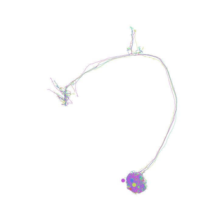
Plot list of neurons as simple 2d

>>> nl = navis.example_neurons()
>>> fig, ax = navis.plot2d(nl, method='2d', view=('x', '-y'))
>>> plt.show() 

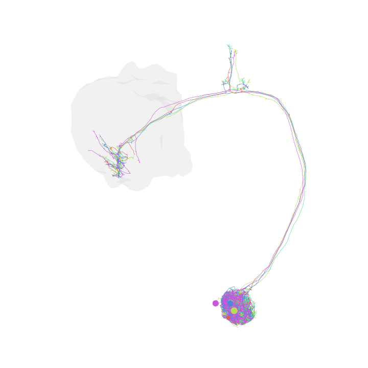
Add a volume

>>> vol = navis.example_volume('LH')
>>> fig, ax = navis.plot2d([nl, vol], method='2d', view=('x', '-y'))
>>> plt.show() 

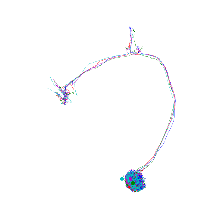
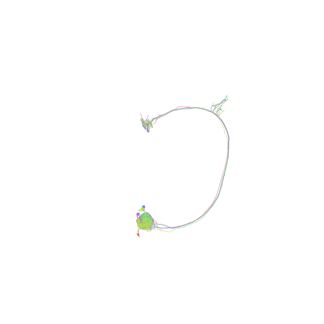
Change neuron colors

>>> fig, ax = navis.plot2d(nl,
...                        method='2d',
...                        view=('x', '-y'),
...                        color=['r', 'g', 'b', 'm', 'c', 'y'])
>>> plt.show() 

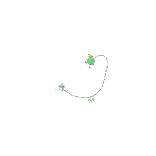
Plot in “fake” 3D

>>> fig, ax = navis.plot2d(nl, method='3d')
>>> plt.show() 
>>> # In an interactive window you can dragging the plot to rotate

Plot in “fake” 3D and change perspective

>>> fig, ax = navis.plot2d(nl, method='3d')
>>> # Change view to frontal (for example neurons)
>>> ax.azim = ax.elev = 90
>>> # Change view to lateral
>>> ax.azim, ax.elev = 180, 180
>>> ax.elev = 0
>>> # Change view to top
>>> ax.azim, ax.elev = 90, 180
>>> # Tilted top view
>>> ax.azim, ax.elev = -130, -150
>>> # Move camera
>>> ax.dist = 6
>>> plt.show() 

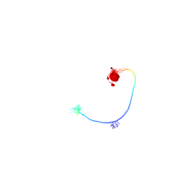
Plot using depth-coloring

>>> fig, ax = navis.plot2d(nl, method='3d', depth_coloring=True)
>>> plt.show() 

To close all figures

>>> plt.close('all')

See the plotting tutorial for more examples.

Returns:: fig, ax
Return type:: matplotlib figure and axis object