NBLAST¶

As of version 0.4.0 navis has a native implementation of NBLAST (Costa et al., 2016) that matches that in R’s nat.nblast.

What is NBLAST?¶

A brief introduction (modified from Jefferis lab’s website):

NBLAST works by decomposing neurons into point and tangent vector representations - so called “dotprops”. Similarity between a given query and a given target neuron is determined by:

1. Find nearest-neighbors¶

For each point + tangent vector of the query neuron, find the closest point + tangent vector on the target neuron (a simple nearest-neighbor search using Euclidean distance).

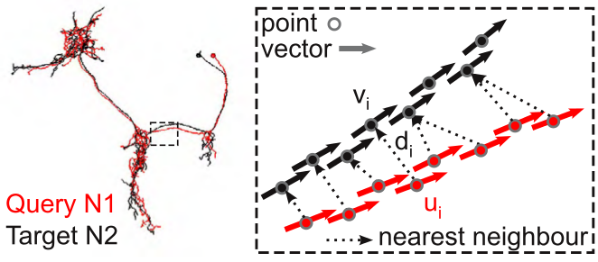
../../_images/NBLAST_neuron_comparison.png

2. Produce a raw score¶

The raw score is a weighted product from the distance $d_{i}$ between the points in each pair and the absolute dot product of the two tangent vectors $| \vec{u_i} \cdot \vec{v_i} |$ .

The absolute dot product is used because the orientation of the tangent vectors has no meaning in our data representation.

A suitable scoring function $f$ was determined empirically (see the NBLAST paper) and is shipped with navis as scoring matrices:

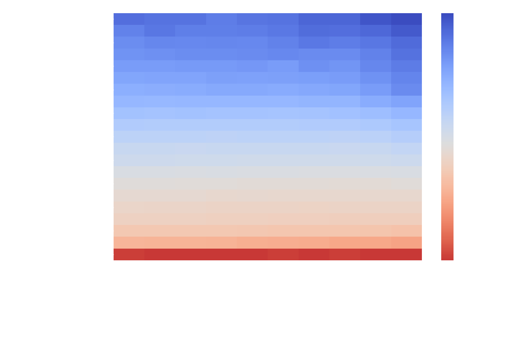
Importantly, these matrices were created using Drosophila neurons from the FlyCircuit light-level dataset which are in microns. Consequently, you should make sure your neurons are in micrometer units too. If you are working on non-insect neurons you might have to play around with the scaling to improve results. Alternatively, you can also produce your own scoring function (see this tutorial).

3. Produce a per-pair score¶

This is done by simply summing up the raw scores over all point + tangent vector pairs.

4. Normalize raw score¶

This step is optional but highly recommended: normalizing the raw score by dividing by the raw score of a self-self comparison of the query neuron.

Summary¶

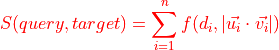
Putting it all together, the formula for the raw score $S$ is:

$S(query,target)=\sum_{i=1}^{n}f(d_{i}, |\vec{u_i} \cdot \vec{v_i}|)$

One important thing to keep in mind is this: the direction of the comparison matters! Consider two very different neurons - one large, one small - that overlap in space. If the small neuron is the query, you will always find a close-by nearest-neighbour among the many points of the large target neuron. Consequently, this small -> large comparison will produce decent NBLAST score. Conversely, the other way around (large -> small) will likely produce a bad NBLAST score because many points in the large neuron are far away from the closests point in the small neuron. In practice, we typically use the mean between those two scores. This is done either by running two nblasts (query -> target and target -> query), or by using the scores parameter of the respective NBLAST function.

Running NBLAST¶

Broadly speaking, there are two applications for NBLAST:

Matching neurons neurons between two datasets
Clustering neurons into morphologically similar groups

Before we get our feet wet some things to keep in mind:

neurons should be in microns as this is what NBLAST’s scoring matrices have been optimized for (see above)
neurons should have similar sampling resolution (i.e. points per unit of cable)
for a ~2x speed boost, install pykdtree library: pip3 install pykdtree (if you are on Linux, make sure to have a look at this Github issue)

OK, let’s get started!

We will use the example neurons that come with navis. These are all of the same type, so we don’t expect to find very useful clusters - good enough to demo though!

# Load example neurons
import navis
nl = navis.example_neurons()

NBLAST works on dotprops - these consist of points and tangent vectors decribing the shape of a neuron and are represented by navis.Dotprops in navis. You can generate those dotprops from skeletons (i.e. TreeNeurons) or meshes (i.e. MeshNeurons) - see navis.make_dotprops() for details.

# Convert neurons into microns (they are 8nm)
nl_um = nl / (1000 / 8)

# Generate dotprops yourself
dps = navis.make_dotprops(nl_um, k=5, resample=False)
nbl = navis.nblast(dps[:3], dps[3:], progress=False)
nbl

	754534424	754538881
1734350788	0.732413	0.769924
1734350908	0.763119	0.753420
722817260	0.742483	0.793841

Painless, wasn’t it? By default, scores are normalized such that 1 is a perfect match (i.e. from a sel-self comparison). We can demonstrate this by running a all-by-all nblast:

aba = navis.nblast_allbyall(dps, progress=False)
aba

	1734350788	1734350908	722817260	754534424	754538881
1734350788	1.000000	0.745189	0.752534	0.732413	0.769924
1734350908	0.734561	1.000000	0.680369	0.763119	0.753420
722817260	0.773701	0.743193	1.000000	0.742483	0.793841
754534424	0.764965	0.767294	0.715226	1.000000	0.784653
754538881	0.760821	0.753727	0.753172	0.763099	1.000000

Let’s run some quick & dirty analysis. In above score matrices, the rows are the queries and the columns are the targets. Forward and reverse scores are never exactly the same.

For hierarchical clustering, however, we need the matrix to be symmetrical. We will therefore use the mean of forward and reverse scores.

aba_mean = (aba + aba.T) / 2

We also need distances instead of similarities!

# Invert to get distances
# Because our scores are normalized, we know the max similarity is 1
aba_dist = 1 - aba_mean
aba_dist

	1734350788	1734350908	722817260	754534424	754538881
1734350788	0.000000	0.260125	0.236882	0.251311	0.234628
1734350908	0.260125	0.000000	0.288219	0.234793	0.246427
722817260	0.236882	0.288219	0.000000	0.271146	0.226493
754534424	0.251311	0.234793	0.271146	0.000000	0.226124
754538881	0.234628	0.246427	0.226493	0.226124	0.000000

from scipy.spatial.distance import squareform
from scipy.cluster.hierarchy import linkage, dendrogram, set_link_color_palette

import matplotlib.pyplot as plt
import matplotlib.colors as mcl
import seaborn as sns

set_link_color_palette([mcl.to_hex(c) for c in sns.color_palette('muted', 10)])

# To generate a linkage, we have to bring the matrix from square-form to vector-form
aba_vec = squareform(aba_dist, checks=False)

# Generate linkage
Z = linkage(aba_vec, method='ward')

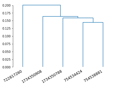
# Plot a dendrogram
dn = dendrogram(Z, labels=aba_mean.columns)

ax = plt.gca()
ax.set_xticklabels(ax.get_xticklabels(), rotation=30, ha='right')

sns.despine(trim=True, bottom=True)

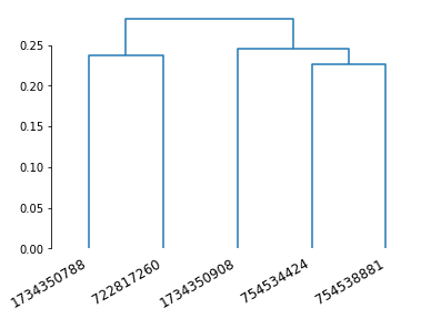
We’ll finish with a notable mention: if you ever want to run a very large NBLAST (talking thousands of neurons) you might want to take a look at navis.nblast_smart().

`navis.nblast`(query[, target, scores, ...])	NBLAST query against target neurons.
`navis.nblast_allbyall`(x[, normalized, ...])	All-by-all NBLAST of inputs neurons.
`navis.nblast_smart`(query[, target, t, ...])	Smart(er) NBLAST query against target neurons.

Another flavour: syNBLAST¶

SyNBLAST is synapse-based NBLAST: instead of turning neurons into dotprops, we use their synapses to perform NBLAST (minus the vector component). This is generally faster because we avoid having to generate dotprops. It also focusses the attention on the synapse-bearing axons and dendrites, effectively ignoring the backbone. This changes the question from “do neurons look the same” to “do neurons have in- and output in the same area”. See navis.synblast() for details.

Let’s try the above but with syNBLAST.

# Note that we still want to use data in microns
# as the scoring function is the same
synbl = navis.synblast(nl_um, nl_um, by_type=True, progress=False)
synbl

	1734350788	1734350908	722817260	754534424	754538881
1734350788	1.000000	0.831690	0.828234	0.820261	0.849559
1734350908	0.831721	1.000000	0.741676	0.857372	0.833785
722817260	0.842672	0.827759	1.000000	0.815891	0.853005
754534424	0.862494	0.853088	0.793840	1.000000	0.866798
754538881	0.845366	0.833463	0.829094	0.844647	1.000000

# Generate the linear vector
aba_vec = squareform(((synbl + synbl.T) / 2 - 1) * -1, checks=False)

# Generate linkage
Z = linkage(aba_vec, method='ward')

# Plot a dendrogram
dn = dendrogram(Z, labels=synbl.columns)

ax = plt.gca()
ax.set_xticklabels(ax.get_xticklabels(), rotation=30, ha='right')

sns.despine(trim=True, bottom=True)

A real-world example¶

The toy data above is not really suited to demonstrate NBLAST because these neurons are of the same type (i.e. we do not expect to see differences).

Let’s try something more elaborate and pull some hemibrain neurons from neuprint. For this you need to install neuprint-python (pip3 install neuprint-python), make a neuPrint account and generate/set an authentication token. Sounds complicated but is all pretty painless - see their documentation for details. There is also a separate navis tutorial on neuprint.

Once that’s done we can get started by importing the neuPrint interface from navis:

import navis.interfaces.neuprint as neu

# Set a client
client = neu.Client('https://neuprint.janelia.org', dataset='hemibrain:v1.2.1')

Next we will fetch all olfactory projection neurons of the lateral lineage using a regex pattern.

pns = neu.fetch_skeletons(neu.NeuronCriteria(type='.*lPN.*', regex=True), with_synapses=True)

# Drop neurons on the left hand side
pns = pns[[not n.name.endswith('_L') for n in pns]]

pns.head()

	type	name	id	n_nodes	n_connectors	n_branches	n_leafs	cable_length	soma	units
0	navis.TreeNeuron	VA5_lPN_R	574032862	4509	2849	739	763	3.023454e+05	9	8 nanometer
1	navis.TreeNeuron	VA5_lPN_R	574037281	4365	2891	719	756	2.994139e+05	19	8 nanometer
2	navis.TreeNeuron	VA5_lPN_R	574374051	4480	3000	751	786	3.098901e+05	6	8 nanometer
3	navis.TreeNeuron	DM5_lPN_R	635416407	2589	1443	330	346	1.972500e+05	1507	8 nanometer
4	navis.TreeNeuron	DM1_lPN_R	542634818	16273	15317	3216	3369	1.167167e+06	15873	8 nanometer

Generate dotprops and convert to microns.

pns_um = pns / (1000 / 8)
pns_dps = navis.make_dotprops(pns_um, k=5)
pns_dps

<class 'navis.core.neuronlist.NeuronList'> containing 54 neurons (0.0B)

	type	name	id	k	units	n_points
0	navis.Dotprops	VA5_lPN_R	574032862	5	1.0 micrometer	4509
1	navis.Dotprops	VA5_lPN_R	574037281	5	1.0 micrometer	4365
...	...	...	...	...	...	...
52	navis.Dotprops	VA7m_lPN_R	5813055180	5	1.0 micrometer	3739
53	navis.Dotprops	DM2_lPN_R	5901222910	5	1.0 micrometer	6484

# Run an all-by-all NBLAST and synNBLAST
pns_nbl = navis.nblast_allbyall(pns_dps, progress=False)
pns_synbl = navis.synblast(pns_um, pns_um, by_type=True, progress=False)

# Generate the linear vectors
nbl_vec = squareform(((pns_nbl + pns_nbl.T) / 2 - 1) * -1, checks=False)
synbl_vec = squareform(((pns_synbl + pns_synbl.T) / 2 - 1) * -1, checks=False)

# Generate linkages
Z_nbl = linkage(nbl_vec, method='ward', optimal_ordering=True)
Z_synbl = linkage(synbl_vec, method='ward', optimal_ordering=True)

# Plot dendrograms
fig, axes = plt.subplots(1, 2, figsize=(12, 5))

dn1 = dendrogram(Z_nbl, no_labels=True, color_threshold=1, ax=axes[0])
dn2 = dendrogram(Z_synbl, no_labels=True, color_threshold=1, ax=axes[1])

axes[0].set_title('NBLAST')
axes[1].set_title('synNBLAST')

sns.despine(trim=True, bottom=True)

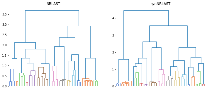
While we don’t know which leaf is which, the structure in both dendrograms looks similar. If we wanted to take it further than that, we could use tanglegram to line up the two clusterings and investigate differences.

But let’s save that for another day and instead do some plotting:

# Generate clusters
from scipy.cluster.hierarchy import fcluster
cl = fcluster(Z_synbl, t=1, criterion='distance')
cl

array([ 6,  6,  6,  8,  8,  8,  3,  8, 15,  2,  2,  2, 14,  7, 13, 10, 14,
        1,  1, 13,  3, 10,  1, 10, 11, 10,  2,  2,  7,  2,  7,  7,  7,  9,
       11,  4,  3,  9,  9,  5,  9,  9, 12, 14, 14, 15, 11, 11, 13,  2,  5,
       12,  5,  8], dtype=int32)

# Now plot each cluster
# For simplicity we are plotting in 2D here
import math

n_clusters = max(cl)
rows = 4
cols = math.ceil(n_clusters / 4)
fig, axes = plt.subplots(rows, cols,
                         figsize=(20, 5 * cols))
# Flatten axes
axes = [ax for l in axes for ax in l]

# Generate colors
pal = sns.color_palette('muted', n_clusters)

for i in range(n_clusters):
    ax = axes[i]
    ax.set_title(f'cluster {i + 1}')
    # Get the neurons in this cluster
    this = pns[cl == (i + 1)]

    navis.plot2d(this, method='2d', ax=ax, color=pal[i], lw=1.5, view=('x', '-z'), alpha=.5)

for ax in axes:
    ax.set_aspect('equal')
    ax.set_axis_off()

    # Set all axes to the same limits
    bbox = pns.bbox
    ax.set_xlim(bbox[0][0], bbox[0][1])
    ax.set_ylim(-bbox[2][1], -bbox[2][0])

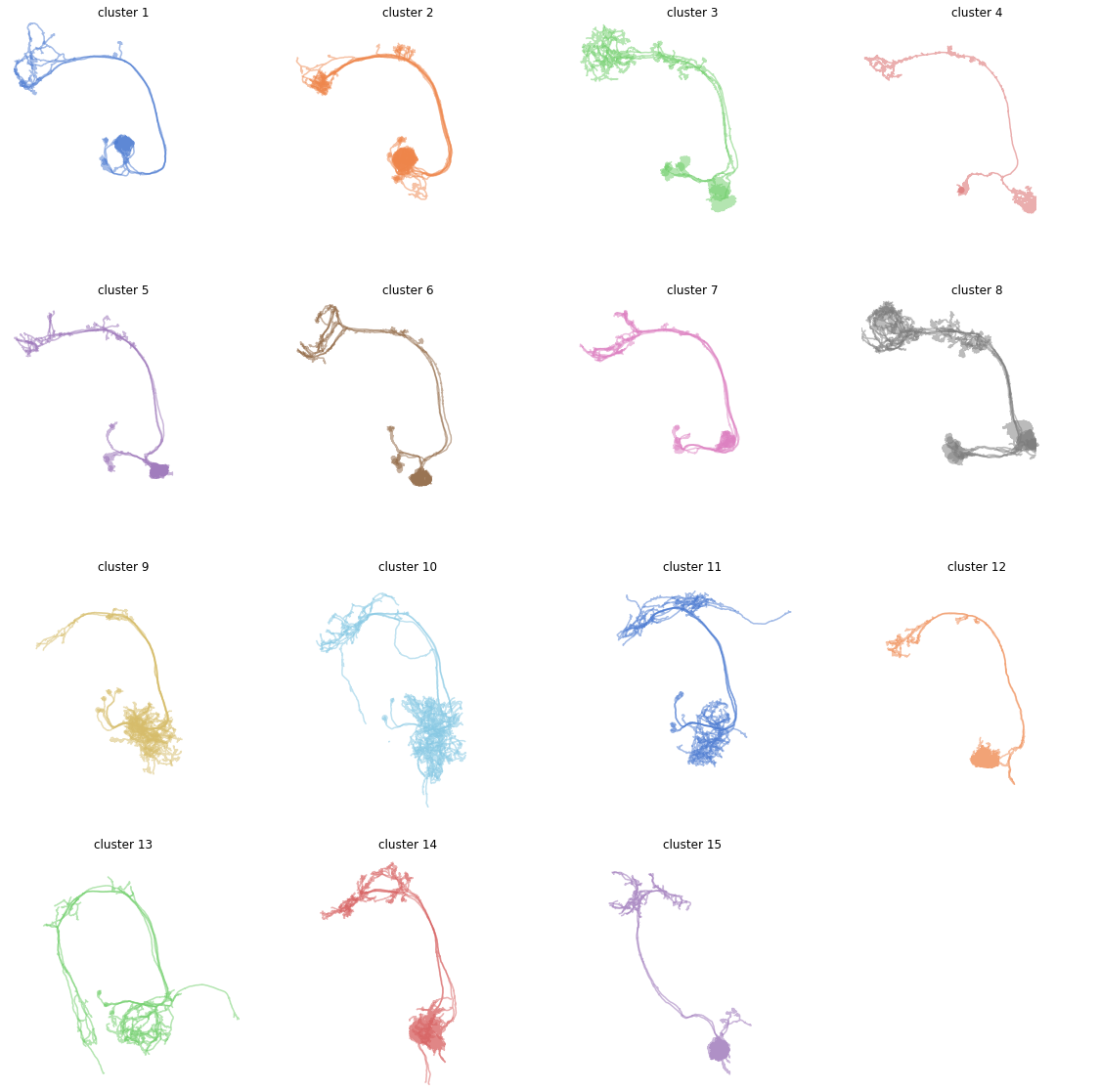
Note how cluster 3 and 8 look odd? That’s because these likely still contain more than one type of neuron. We should probably have gone with a slightly finer clustering. But this little demo should be enough to get you started!

References¶

NBLAST: Rapid, Sensitive Comparison of Neuronal Structure and Construction of Neuron Family Databases. Costa M, Manton JD, Ostrovsky AD, Prohaska S, Jefferis GSXE. Neuron. 2016 doi: 10.1016/j.neuron.2016.06.012