NBLAST against FlyCircuit
If you work with Drosophila, chances are you have heard of FlyCircuit. It’s a collection of ~16k single neuron clones published by Chiang et al. (2010).
For R, there is a package containing dotprops and meta data for these neurons: nat.flycircuit. This does not yet exist for Python. However, it’s still reasonably straight forward to run an NBLAST against the entire flycircuit dataset in Python:
First you need to download flycircuit dotprops from Zenodo (850Mb). Next, unzip the archive containing the dotprops as CSV files. Now we can load them into navis (adjust filepaths as required):
import navis
import pandas as pd

from pathlib import Path
from tqdm import tqdm
def load_dotprops_csv(fp):
    """Load dotprops from CSV files in filepath `fp`."""
    # Turn into a path object
    fp = Path(fp).expanduser()

    # Go over each CSV file
    files = list(fp.glob('*.csv'))
    dotprops = []
    for f in tqdm(files, desc='Loading dotprops', leave=False):
        # Read file
        csv = pd.read_csv(f)

        # Each row is a point with associated vector
        pts = csv[['pt_x', 'pt_y', 'pt_z']].values
        vect = csv[['vec_x', 'vec_y', 'vec_z']].values

        # Turn into a Dotprops
        dp = navis.Dotprops(points=pts, k=20, vect=vect, units='1 micron')

        # Use filename as ID/name
        dp.name = dp.id = f.name[:-4]

        # Add this dotprop to the list before moving on to the next
        dotprops.append(dp)

    return navis.NeuronList(dotprops)

fc_dps = load_dotprops_csv('~/Downloads/flycircuit_dotprops')
fc_dps
| type | name | id | k | units | n_points | |
|---|---|---|---|---|---|---|
| 0 | navis.Dotprops | DvGlutMARCM-F1822_seg2 | DvGlutMARCM-F1822_seg2 | 20 | 1 micrometer | 87 |
| 1 | navis.Dotprops | DvGlutMARCM-F002216_seg001 | DvGlutMARCM-F002216_seg001 | 20 | 1 micrometer | 2574 |
| ... | ... | ... | ... | ... | ... | ... |
| 16127 | navis.Dotprops | GadMARCM-F000020_seg001 | GadMARCM-F000020_seg001 | 20 | 1 micrometer | 477 |
| 16128 | navis.Dotprops | DvGlutMARCM-F1720_seg1 | DvGlutMARCM-F1720_seg1 | 20 | 1 micrometer | 941 |
To avoid having to re-generate these dotprops, you could consider pickling them:
In the future you can then reload the dotprops like so (much faster):
Note: The names/ids correspond to the flycircuit gene + clone names!
fc_dps[0]
| type | navis.Dotprops |
|---|---|
| name | FruMARCM-M002262_seg001 |
| id | FruMARCM-M002262_seg001 |
| k | 5 |
| units | 1 micrometer |
| n_points | 4121 |
In case your query neurons are in a different brain space, you can use navis-flybrains to convert them to flycircuit’s FCWB space.
For demonstration purposes we will use the example neurons - olfactory DA1 projection neurons from the hemibrain connectome - that ship with navis.
# Load some of the example neurons
n = navis.example_neurons(3)
# Convert from hemibrain (JRCFIB2018Fraw) to FCWB space
import flybrains

n_fcwb = navis.xform_brain(n, source='JRCFIB2018Fraw', target='FCWB')
Transform path: JRCFIB2018Fraw -> JRCFIB2018F -> JRCFIB2018Fum -> JRC2018F -> FCWB
# A sanity check to make sure the transform worked
fig, ax = navis.plot2d([n_fcwb, flybrains.FCWB])

# Rotate to front view
ax.elev = -90

# Zoom in a little
ax.dist = 4
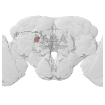
# Mirror neurons from the right to the left
# (FlyCircuit neurons are supposed to all be on the left)
n_fcwb_mirr = navis.mirror_brain(n_fcwb, template='FCWB')
# Convert to dotprops
n_dps = navis.make_dotprops(n_fcwb_mirr, resample=1, k=None)
# Run a "smart" NBLAST to get the top hits
# (ignore the warning about data not being in microns - that's a rounding error from the transform)
scores = navis.nblast_smart(query=n_dps, target=fc_dps, scores='mean', progress=False)
scores.head()
| FruMARCM-M002262_seg001 | FruMARCM-M002262_seg002 | FruMARCM-M002278_seg001 | FruMARCM-M002287_seg001 | FruMARCM-M002507_seg001 | FruMARCM-M002522_seg001 | FruMARCM-M002578_seg001 | FruMARCM-M002578_seg002 | FruMARCM-M002579_seg001 | FruMARCM-M002579_seg002 | ... | DvGlutMARCM-F594-X2_seg1 | DvGlutMARCM-F594-X2_seg2 | DvGlutMARCM-F595_seg1 | DvGlutMARCM-F596_seg1 | DvGlutMARCM-F597_seg1 | DvGlutMARCM-F598_seg1 | DvGlutMARCM-F599_seg1 | DvGlutMARCM-F599_seg2 | DvGlutMARCM-F600-X2_seg1 | DvGlutMARCM-F600-X2_seg2 | |
|---|---|---|---|---|---|---|---|---|---|---|---|---|---|---|---|---|---|---|---|---|---|
| 1734350788 | -0.260213 | -0.200286 | -0.645926 | -0.639277 | -0.663507 | -0.451059 | -0.229996 | -0.604237 | -0.705247 | -0.307929 | ... | -0.881092 | -0.648820 | -0.660410 | 0.118524 | -0.315490 | -0.671891 | -0.499438 | -0.882007 | -0.882510 | -0.880825 |
| 1734350908 | -0.267769 | -0.191842 | -0.655194 | -0.623617 | -0.679471 | -0.459428 | -0.233066 | -0.607806 | -0.715372 | -0.310166 | ... | -0.881365 | -0.654605 | -0.669929 | 0.113844 | -0.316001 | -0.682929 | -0.505106 | -0.881421 | -0.881361 | -0.882250 |
| 722817260 | -0.270642 | -0.170228 | -0.680244 | -0.667571 | -0.670850 | -0.431723 | -0.236943 | -0.634743 | -0.704928 | -0.298078 | ... | -0.881398 | -0.649228 | -0.659683 | 0.132546 | -0.317336 | -0.627997 | -0.503828 | -0.882124 | -0.881570 | -0.881419 |
3 rows × 16129 columns
# Find the top hits for each of our query neurons
import numpy as np

for dp in n_dps:
    hit = scores.columns[np.argmax(scores.loc[dp.id].values)]
    sc = scores.loc[dp.id].values.max()
    print(f'Top hit for {dp.id}: {hit} ({sc:.3f})')
Top hit for 1734350788: FruMARCM-F001496_seg001 (0.778)
Top hit for 1734350908: FruMARCM-F001496_seg001 (0.744)
Top hit for 722817260: FruMARCM-F001496_seg001 (0.792)
Conveniently all of our query neurons have the same top match (they are all from the same cell type after all): FruMARCM-F001496_seg001
# Let's co-visualize:
# Queries in red, hit in black
fig, ax = navis.plot2d([n_fcwb_mirr, fc_dps.idx['FruMARCM-F001496_seg001']],
                       color=['r'] * len(n_fcwb_mirr) + ['k'])
ax.elev = -90
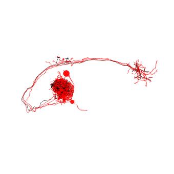
Looking good!