R and the nat libraries

NAVis is inspired by the excellent nat (NeuroAnatomy Toolbox) ecosystem by Greg Jefferis . While there is parity in major features between the navis ecosystem and the “natverse”, it can sometimes be useful to access R functions directly.

Fortunately, Python and R play very nicely together - see this brilliant blog post. Hence, NAVis has functions for converting from/to nat datatypes and basic wrappers for some of the most useful nat functions. This section will teach you the basics of how to use R and NAVis. But first, we have to make sure you are all set:

Setting up

Using R from within Python requires rpy2. rpy2 is not automatically installed alongside NAVis. That’s because it fails to install if R is not already present on your system. Here is what you need to do:

1. Install R.
   You can either install just R or install it along with R Studio (recommended).
2. Install rpy2
   This should do the trick:

   pip3 install rpy2

   Check out rpy2's documentation if you are running into issues.
3. Install R packages.
   NAVis has wrappers for the nat (NeuroAnatomy Toolbox) ecosystem by Greg Jefferis. Please make sure to install:
   1. nat - core package for morphological analysis of neurons
   2. nat.nblast - morphological similarity
   3. elmr - bridging between EM and light level data
   4. rcatmaid - interface with CATMAID
   5. flycircuit - interface with the flycircuit database for fly neurons
   6. nat.templatebrains and nat.flybrains - bridging between different light level template brains

You are ready to go! On a fundamental level, you can now use every single R function from within Python - check out the rpy2 documentation.

Quickstart

import navis

navis.set_pbars(hide=True, jupyter=False)

from navis.interfaces import r

import matplotlib.pyplot as plt

from rpy2.robjects.packages import importr
import rpy2.robjects as robjects

Load nat as module

nat = importr('nat')

Run one of the nat examples in Python

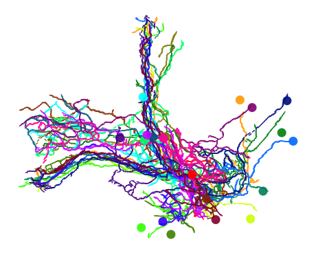
# Get neurons (Drosophila Kenyon cells) shipped with nat
kcs20 = robjects.r('kcs20')

head = robjects.r('head')

head(kcs20)

R/rpy2 DataFrame (6 x 14)

gene_name	Name	idid	...	cluster	idx	type
'FruM...	'fru-...	1024.000000	...	9	156	gamma
'GadM...	'Gad1...	10616.000000	...	70	1,519	gamma
'GadM...	'Gad1...	8399.000000	...	57	1,132	ab
'GadM...	'Gad1...	10647.000000	...	71	1,535	apbp
'FruM...	'fru-...	9758.000000	...	64	1,331	ab
'FruM...	'fru-...	6182.000000	...	44	795	ab

Convert the Kenyon cells to NAVis DotProps

kcs20_py = r.dotprops2py(kcs20)
kcs20_py.head()

	gene_name	Name	idid	soma_side	flipped	Driver	Gender	X	Y	Z	exemplar	cluster	idx	type	points
0	FruMARCM-M001205_seg002	fru-M-500112	1024.0	L	0	fru-Gal4	M	361.484872	95.044800	84.102594	FruMARCM-M001205_seg002	9	156	gamma	x y z x_v...
1	GadMARCM-F000122_seg001	Gad1-F-900005	10616.0	L	0	Gad1-Gal4	F	367.833167	105.867548	94.734459	GadMARCM-F000122_seg001	70	1519	gamma	x y z x_v...
2	GadMARCM-F000050_seg001	Gad1-F-100010	8399.0	R	1	Gad1-Gal4	F	382.827911	61.732132	97.280571	GadMARCM-F000050_seg001	57	1132	ab	x y z x_ve...
3	GadMARCM-F000142_seg002	Gad1-F-300043	10647.0	L	0	Gad1-Gal4	F	349.591724	78.189859	96.692797	GadMARCM-F000142_seg002	71	1535	apbp	x y z x_ve...
4	FruMARCM-F000270_seg001	fru-F-400045	9758.0	L	0	fru-Gal4	F	387.523611	114.803444	87.841563	FruMARCM-F000270_seg001	64	1331	ab	x y z x_v...

Plot them

fig, ax = navis.plot2d(kcs20_py, linewidth=1.5)

Data conversion

navis.interfaces.r provides functions to convert data from Python to R:

1. navis.interfaces.r.data2py() converts general data from R to Python

2. navis.interfaces.r.neuron2py() converts R neuron or neuronlist objects to Python navis.TreeNeuron and navis.NeuronList, respectively

3. navis.interfaces.r.neuron2r() converts navis.TreeNeuron or navis.NeuronList to R neuron or neuronlist objects

4. navis.interfaces.r.dotprops2py() converts R dotprop objects to pandas DataFrame that can be passed to navis.plot.plot3d()

R NBLAST

NAVis has a native (i.e. pure Python) implementation of NBLAST (see this Tutorial) that matches the one in nat. While I recommend that you use the Python implementation, you can also use the nat interface to run the R NBLAST:

navis.interfaces.r.nblast(query[, target, ...])	NBLAST using R's nat.nblast::nblast.
navis.interfaces.r.nblast_allbyall(x[, ...])	All-by-all NBLAST using R's nat.nblast::nblast_allbyall.
navis.interfaces.r.NBLASTresults(results, ...)	Class holding NBLAST results and wrappers that allow easy plotting.

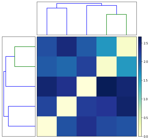
All-by-all nblast

Comparing neurons which are already in the same brain space is straight forward:

nl = navis.example_neurons()

# Note that we are converting to microns as NBLAST is optimized for that resolution
nbl = r.nblast_allbyall(nl, micron_conversion=1/1000, resample=1)

fig = nbl.plot_matrix()

INFO  : Use matplotlib.pyplot.show() to render figure. (navis)

NBLAST against databases

In this example we will nblast one of our example Drosophila neurons against the flycircuit database of single cell clones.

This is a two step process in which the neuron is first transformed from it’s original brain space (FAFB14) into the flycircuit template space (FCWB) and then blasted against the entire database of skeletonized flycircuit clones.

This requires you to have the R flycircuit and nat.templatebrains packages installed.

n = navis.example_neurons(1)

# Get the flycircuit database
datadir = robjects.r('getOption("flycircuit.datadir")')[0]
fc = robjects.r(f'read.neuronlistfh("{datadir}/dpscanon.rds")')

nbl = r.nblast(n, db=fc, xform='FAFB14->FCWB', resample=1, mirror=True)

INFO  : Blasting neuron... (navis)
INFO  : Blasting done in 67.3 seconds (navis)

Show the top results

nbl.results.head()

	gene_name	forward_score	reverse_score	mu_score
0	DvGlutMARCM-F002430_seg001	0.614162	0.632155	0.623158
1	FruMARCM-M002373_seg002	0.603885	0.681603	0.642744
2	dTdc2MARCM-F000115_seg001	0.588686	-0.498178	0.045254
3	ChaMARCM-F000725_seg001	0.566431	0.676217	0.621324
4	GadMARCM-F000709_seg001	0.565479	0.566549	0.566014

Plot the top 2 hits ontop of the query neuron (black).

fig = nbl.plot3d(hits=2, width=1000)