Transformations¶

Introduction¶

As of version 0.5.0, navis includes functions that let you transform and mirror spatial data (e.g. neurons). This new functionality broadly splits into high and low level functions. In this tutorial, we will start by exploring the higher level functions that most users will use and then take a sneak peak at the low level functions.

At the moment, navis supports the following transform types:

CMTK warp transforms
Hdf5 deformation fields
Elastix transforms
landmark-based thin spline plate transforms
affine transforms

flybrains¶

Since navis brings the utility but does not ship with any transforms, we have to either generate those ourselves or get them elsewhere. Here, we will showcase the flybrains library that provides a number of different transforms directly to navis. Setting up and registering your own custom transforms will be discussed further down.

First, you need to get flybrains. Please follow the instructions to install and download the bridging registrations before you continue.

import flybrains

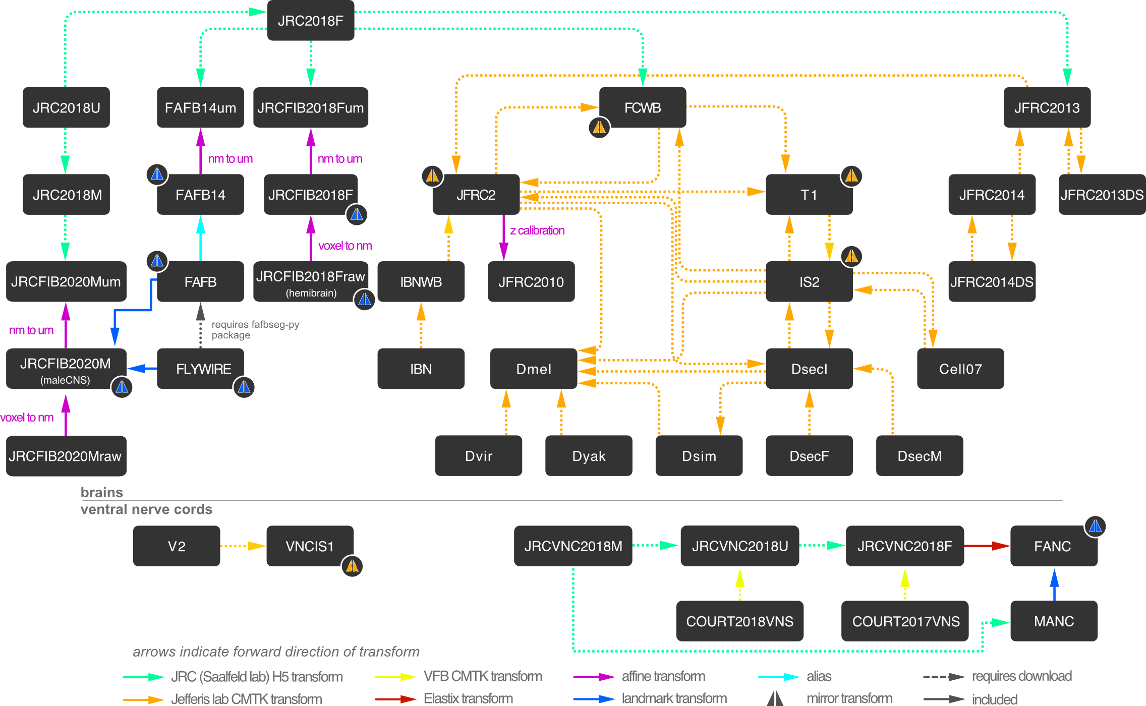
Importing flybrains automatically registers the transforms with navis. That allows navis to plot a sequence of bridging transformations to map between these template spaces.

In addition to those bridging transforms, flybrains also contains mirror registrations (we will cover those later), meta data and meshes for the template brains:

# This is the Janelia "hemibrain" template brain
flybrains.JRCFIB2018F

Template brain
--------------
Name: JRCFIB2018F
Short Name: JRCFIB2018F
Type: None
Sex:  None
Dimensions: NA
Voxel size:
  x = 0.008 m
  y = 0.008 i
  z = 0.008 c
Bounding box (m):
  NA
Description: Calibrated version of Janelia FIB hemibrain dataset
DOI: https://doi.org/10.1101/2020.01.21.911859

import navis

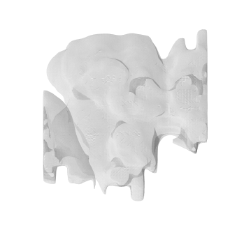
# This is the hemibrain neuropil surface mesh
fig, ax = navis.plot2d(flybrains.JRCFIB2018F)
ax.azim, ax.elev = -90, 180

You can check the registered transforms like so:

navis.transforms.registry.summary()

	source	target	transform	type	invertible	weight
0	IBNWB	JFRC2	CMTKtransform with 1 transform(s)	bridging	True	1
1	JFRC2013	JFRC2013DS	CMTKtransform with 1 transform(s)	bridging	True	1
2	JFRC2013DS	JFRC2013	CMTKtransform with 1 transform(s)	bridging	True	1
3	JFRC2014	JFRC2013	CMTKtransform with 1 transform(s)	bridging	True	1
4	JFRC2	T1	CMTKtransform with 1 transform(s)	bridging	True	1
...	...	...	...	...	...	...
97	JRCFIB2018Fraw	JRCFIB2018F	<navis.transforms.affine.AffineTransform objec...	bridging	True	1
98	JRCFIB2018F	JRCFIB2018Fum	<navis.transforms.affine.AffineTransform objec...	bridging	True	1
99	FAFB14um	FAFB14	<navis.transforms.affine.AffineTransform objec...	bridging	True	1
100	FAFB	FAFB14	<navis.transforms.base.AliasTransform object a...	bridging	True	1
101	JFRC2	JFRC2010	<navis.transforms.affine.AffineTransform objec...	bridging	True	1

102 rows × 6 columns

Using `xform_brain`¶

For high level transforming, you will want to use navis.xform_brain(). This function takes a source and target argument tries to find a bridging sequence that gets you to where you want. Let’s try it out:

Incidentally, the example neurons that navis ships with are from the Janelia hemibrain project and are therefore in JRCFIB2018raw (raw = 8nm voxel coordinates). We will be using those but there is nothing stopping you from using navis' interface with neuPrint (tutorial) to fetch your favourite hemibrain neurons and transform those.

# Load the example hemibrain neurons (JRCFIB2018raw space)
nl = navis.example_neurons()
nl

	type	name	id	n_nodes	n_connectors	n_branches	n_leafs	cable_length	soma	units
0	navis.TreeNeuron	1734350788	1734350788	4465	None	603	None	266458.0000	[4176]	8 nanometer
1	navis.TreeNeuron	1734350908	1734350908	4845	None	733	None	304277.0000	[6]	8 nanometer
2	navis.TreeNeuron	722817260	722817260	4336	None	635	None	274910.5625	None	8 nanometer
3	navis.TreeNeuron	754534424	754534424	4702	None	697	None	286743.0000	[4]	8 nanometer
4	navis.TreeNeuron	754538881	754538881	4890	None	626	None	291435.0000	[703]	8 nanometer

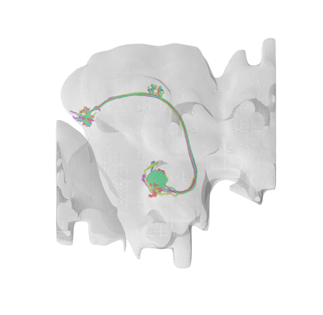
fig, ax = navis.plot2d([nl, flybrains.JRCFIB2018Fraw], linewidth=2, figsize=(8, 8))
ax.azim, ax.elev = -90, 180

Let’s say we want these neurons in JRC2018F template space. Before we do the actual transform it’s useful to quickly check above bridging graph to see what we expect to happen:

First, we know that we are starting in JRCFIB2018Fraw space. From there, there is are two simple affine transforms to go from voxels to nanometers and from nanometers to micrometers. Once we are in micrometers, we can use a Hdf5 transform generated by the Saalfeld lab to map to JRC2018F (Bogovic et al., 2019). Note that the arrows in the bridging graph indicate the transforms’ forward directions but they can all be inversed to traverse the graph.

OK, with that out of the way:

xf = navis.xform_brain(nl, source='JRCFIB2018Fraw', target='JRC2018F')

Transform path: JRCFIB2018Fraw->JRCFIB2018F->JRCFIB2018Fum->JRC2018F

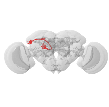
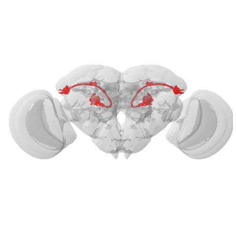
Painless, wasn’t it? Let’s see if it worked:

# Plot the transformed neurons and the JRC2018F template brain
fig, ax = navis.plot2d([xf, flybrains.JRC2018F], linewidth=2, color='r', figsize=(8, 8))
ax.azim, ax.elev = -90, -90
ax.dist = 5

Worked like a charm! I highly recommend you read through the documentation for navis.xform_brain() and check out the parameters you can use to fine-tune it.

Using `mirror_brain`¶

Another useful type of transform is mirroring using navis.mirror_brain(). The way this works is this:

Reflect coordinates about the midpoint of the mirror axis (affine transformation)
Apply a warping transformation to compensate for e.g. left/right asymmetries

For the first step, we need to know the length of the mirror axis. This is why - similar to having registered transforms - we need to have meta data about the template space (i.e. the bounding box) available to navis.

The second step is optional. For example, JRC2018F and JRC2018U are templates generate from averaging multiple fly brains and are therefore already mirror symmetrical. flybrains does include some mirror transforms though: e.g. for FCWB, VNCIS1 or JFRC2.

Since our neurons are already in JRC2018F space, let’s try mirroring them:

mirrored = navis.mirror_brain(xf, template='JRC2018F')

fig, ax = navis.plot2d([xf, mirrored, flybrains.JRC2018F], linewidth=2, color='r', figsize=(8, 8))
ax.azim, ax.elev = -90, -90
ax.dist = 5

Perfect! As noted above, this only works if the template is registered with navis and if it contains info about its bounding box. If you only have the bounding box at hand but no template brain, check out the lower level function navis.transforms.mirror().

Low-level functions¶

Let’s assume you want to add your own transforms. There are four different transform types:

`navis.transforms.affine.AffineTransform`(matrix)	Affine transformation of 3D spatial data.
`navis.transforms.cmtk.CMTKtransform`(regs[, ...])	CMTK transforms of 3D spatial data.
`navis.transforms.h5reg.H5transform`(f[, ...])	Hdf5 transform of 3D spatial data.
`navis.transforms.thinplate.TPStransform`(...)	Thin Plate Spline transforms of 3D spatial data.

To show you how to use them, we will create a new thin plate spline transform using TPStransform. If you look at the bridging graph again, you might note the “FAFB14” template brain: it stands for “Full Adult Fly Brain” and this is is the 14th registration of the data. We will use landmarks to generate a mapping between this 14th and the previous 13th iteration.

First grab the landmarks from the Saalfeld’s lab elm repository:

import pandas as pd

# These landmarks map betweet FAFB (v14 and v13) and a light level template
# We will use only the v13 and v14 landmarks
landmarks_v14 = pd.read_csv('https://github.com/saalfeldlab/elm/raw/master/lm-em-landmarks_v14.csv', header=None)
landmarks_v13 = pd.read_csv('https://github.com/saalfeldlab/elm/raw/master/lm-em-landmarks_v13.csv', header=None)

# Name the columns
landmarks_v14.columns = landmarks_v13.columns = ["label", "use", "lm_x","lm_y","lm_z", "fafb_x","fafb_y","fafb_z"]

landmarks_v13.head()

	label	use	lm_x	lm_y	lm_z	fafb_x	fafb_y	fafb_z
0	Pt-1	True	571.400083	38.859963	287.059544	525666.465856	172470.413167	80994.733289
1	Pt-2	True	715.811344	213.299356	217.393493	595391.597008	263523.121958	84156.773677
2	Pt-3	True	513.002196	198.001970	217.794090	501716.347872	253223.667163	98413.701578
3	Pt-6	True	867.012542	31.919253	276.223437	670999.903156	179097.916778	67561.691416
4	Pt-7	True	935.210895	234.229522	351.518068	702703.909963	251846.384054	127865.886146

Now we can use those landmarks to generate a thin plate spine transform:

from navis.transforms.thinplate import TPStransform

tr = TPStransform(landmarks_source=landmarks_v14[["fafb_x","fafb_y","fafb_z"]].values,
                  landmarks_target=landmarks_v13[["fafb_x","fafb_y","fafb_z"]].values)

# navis.transforms.MovingLeastSquaresTransform has similar properties

The transform has a method that we can use to transform points but first we need some data in FAFB 14 space:

# Transform our neurons into FAFB 14 space
xf_fafb14 = navis.xform_brain(nl, source='JRCFIB2018Fraw', target='FAFB14')

Transform path: JRCFIB2018Fraw->JRCFIB2018F->JRCFIB2018Fum->JRC2018F->FAFB14um->FAFB14

Now let’s see if we can use the v14 -> v13 transform:

# Transform the nodes of the first two neurons
pts_v14 = xf_fafb14[:2].nodes[['x', 'y', 'z']].values

# The actual transform
pts_v13 = tr.xform(pts_v14)

Quick check how the v14 and v13 coordinates compare

fig, ax = navis.plot2d(pts_v14, scatter_kws=dict(c='k'))
_ = navis.plot2d(pts_v13, scatter_kws=dict(c='r'), ax=ax)
ax.azim = ax.elev = -90

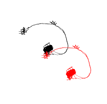
So that did something… to be honest, I’m not sure what to expect for the FAFB 14->13 transform but let’s assume this is correct and move on.

Next, we will register this new transform with navis so that we can use it with higher level functions:

# Register the transform
navis.transforms.registry.register_transform(tr, source='FAFB14', target='FAFB13', transform_type='bridging')

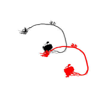
Now that’s done we can use FAFB13 with navis.xform_brain():

# Transform our neurons into FAFB 14 space
xf_fafb13 = navis.xform_brain(xf_fafb14, source='FAFB14', target='FAFB13')

Transform path: FAFB14->FAFB13

fig, ax = navis.plot2d(xf_fafb14, c='k')
_ = navis.plot2d(xf_fafb13, c='r', ax=ax, lw=1.5)
ax.azim = ax.elev = -90

For completeness, lets also have a quick look at registering additional template brains.

Template brains are represented in navis as navis.transforms.templates.TemplateBrain and there is currently no canonical way of constructing them: you can associate as much or as little data with them as you like. However, for them to be useful they should have a name, a label and a boundingbox property.

Minimally, you could do something like this:

# Construct template brain from base class
my_brain = navis.transforms.templates.TemplateBrain(name='My template brain',
                                                    label='my_brain',
                                                    boundingbox=[[0, 100], [0, 100], [0, 100]])

# Register with navis
navis.transforms.registry.register_templatebrain(my_brain)

# Now you can use it with mirror_brain:
import numpy as np
pts = np.array([[10, 10, 10]])
pts_mirrored = navis.mirror_brain(pts, template='my_brain')

# Plot the points
fig, ax = navis.plot2d(pts, scatter_kws=dict(c='k', alpha=1, s=50))
fig, ax = navis.plot2d(pts_mirrored, scatter_kws=dict(c='r', alpha=1, s=50), ax=ax)

While this is a working solution, it’s not very pretty: for example, my_brain does have the default docstring and no fancy string representation (e.g. for print(my_brain)). I highly recommend you take a look at how flybrains constructs the templates.

Acknowledgments

Much of the transform module is modelled after functions written by Greg Jefferis for the natverse. Likewise, flybrains is a port of data collected by Greg Jefferis for nat.flybrains and nat.jrcbrains.