This tutorial will give you an impression of how to process and manipulate your neurons’ morphology. See the API reference for a complete list of available functions.
As you might imagine some manipulations (e.g. smoothing or simplification) will work on all/most neuron types while others will only work on specific types. For example rerooting only makes sense on a TreeNeuron.
The rule of thumb is this: if a function is called e.g. simplify_neuron it should work with multiple if not all neuron types while specialized functions will be called e.g. reroot_skeleton. So depending on what data you are working with and what you want to get out of it, you might have to explicitly convert between neuron types. See the respective function’s docstring for details!
Rerooting
TreeNeurons are hierarchical trees and as such typically have a single “root” node (fragmented neurons will have multiple roots). The root is important because it is used as the reference/origin for a bunch of analyses such as Strahler order. Typically, you want the root to be the soma. Because the root is so important, TreeNeuron can be rerooted:
import navis

n = navis.example_neurons(1, kind='skeleton')
print(n.soma)
[4177]
.soma returns the node ID of the soma (if there is one) and can be used to reroot
navis.reroot_skeleton(n, n.soma)
| type | navis.TreeNeuron |
|---|---|
| name | DA1_lPN_R |
| id | 1734350788 |
| n_nodes | 4465 |
| n_connectors | 2705 |
| n_branches | 598 |
| n_leafs | 619 |
| cable_length | 266476.875 |
| soma | [4177] |
| units | 8 nanometer |
| created_at | 2022-07-27 21:16:48.240027 |
| id | 1734350788 |
| origin | /Users/philipps/Google Drive/Cloudbox/Github/n... |
Note that the root is implicitly also important for MeshNeuron because we’re using their skeletons for a couple operations/analyses.
Simplifying
If you work with large lists of neurons you may want to downsample/simplifiy before e.g. trying to plot them. This is one of the things that - in principle work - with all neuron types. The implementation, however, depends on the neuron type. Lookup the respective function’s help (e.g. via the API) for details.
For TreeNeurons downsampling means skipping N nodes (here 10):
sk = navis.example_neurons(n=1, kind='skeleton')
print(sk.n_nodes)
4465
sk_downsampled = navis.downsample_neuron(sk, downsampling_factor=10, inplace=False)
print(sk_downsampled.n_nodes)
1304
For MeshNeurons downsampling will reduce the number of faces by a factor of N:
me = navis.example_neurons(n=1, kind='mesh')
print(me.n_faces)
13054
me_downsampled = navis.downsample_neuron(me, downsampling_factor=10, inplace=False)
print(me_downsampled.n_faces)
1474
Note
Under the hood downsample_neuron() calls simplify_mesh() for MeshNeurons.
That function then requires one of the supported backends for mesh operations to be installed: Blender
3D, pymeshlab or open3d.
TreeNeurons can also be “resampled” (up or down) to a given resolution (i.e. distance between nodes):
sk = navis.example_neurons(n=1, kind='skeleton')
print(sk.sampling_resolution * sk.units)
477.4501679731243 nanometer
# Note that we can provide a unit ("1 micron") here because our neuron has units set
sk_resampled = navis.resample_skeleton(sk, resample_to='1 micron', inplace=False)
print(sk_resampled.sampling_resolution * sk_resampled.units)
1072.2341923485653 nanometer
Let’s visualize what we did there:
import matplotlib.pyplot as plt

nodes_original = sk.nodes[['x', 'y' ,'z']].values
nodes_downsampled = sk_downsampled.nodes[['x', 'y' ,'z']].values
nodes_resampled = sk_resampled.nodes[['x', 'y' ,'z']].values

fig, axes = plt.subplots(1, 3, figsize=(18, 5))

_ = navis.plot2d(nodes_original, method='2d', view=('x', '-z'), scatter_kws=dict(c='blue'), ax=axes[0])
_ = navis.plot2d(nodes_resampled, method='2d', view=('x', '-z'), scatter_kws=dict(c='red'), ax=axes[1])
_ = navis.plot2d(nodes_downsampled, method='2d', view=('x', '-z'), scatter_kws=dict(c='green'), ax=axes[2])

for ax, title in zip(axes, ['Original', 'Resampled to 1um', 'Downsampled 10x']):
    ax.set_title(title, color='lightgrey')
    ax.set_axis_off()

plt.show()
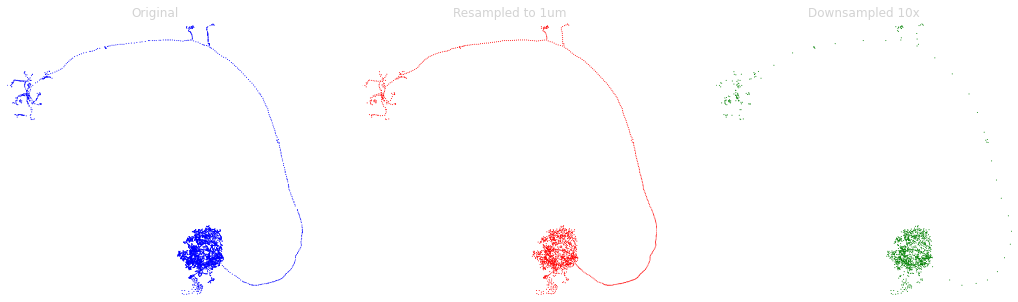
As you can see the resampling increased the node density in the backbone and decreased it in the finer neurites to bring things on par. Downsampling just thinned out the nodes across the board.
Note
Resampling has a caveat you need to be aware of: nodes are not merely moved around to match the desired resolution - they are regenerated from scratch. As consequence, the original node IDs are - with a few exceptions - all gone.
Smoothing
Smoothing is one of those things that work on all neurons but the approaches are so vastly different that there are separate functions: navis.smooth_skeleton(), navis.smooth_mesh() and navis.smooth_voxels():
# smooth_skeleton uses a rolling window along the linear segments
sk = navis.example_neurons(n=1, kind='skeleton')
sk_smoothed = navis.smooth_skeleton(sk, window=5, inplace=False)
# smooth_mesh uses a iterative rounds of Laplacian smoothing
me = navis.example_neurons(n=1, kind='mesh')
me_smoothed = navis.smooth_mesh(me, iterations=5, inplace=False)
Cutting & Pruning
Cutting and pruning work best if there is a sense of topology which implicitly requires a skeleton. Many functions will also work on MeshNeurons though. That’s because the operation is performed on their skeleton and changes are propagated back to the mesh. Fair warning though: this may not be perfect (e.g. the resulting mesh might not be watertight) - should be good enough for a first pass though.
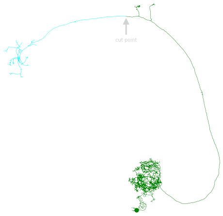
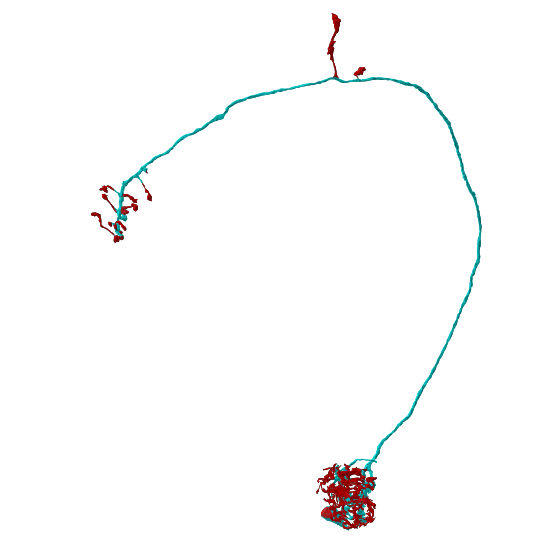
Let’s start with something easy: cutting a skeleton in two at a given node.
# Load the neuron
n = navis.example_neurons(1, kind='skeleton')

# Pick a node ID
cut_node_id = n.nodes.node_id.values[333]
distal, proximal = navis.cut_skeleton(n, cut_node_id)
Plot the two fragments:
# Note that we are using method='2d' here because that makes annotating the plot easier
fig, ax = distal.plot2d(color='cyan', method='2d', view=('x', '-z'))
fig, ax = proximal.plot2d(color='green', ax=ax, method='2d', view=('x', '-z'))

# Annotate cut point
cut_coords = distal.nodes.set_index('node_id').loc[distal.root, ['x', 'z']].values[0]
ax.annotate('cut point',
            xy=(cut_coords[0], -cut_coords[1]),
            color='lightgrey',
            xytext=(cut_coords[0], -cut_coords[1]-2000), va='center', ha='center',
            arrowprops=dict(shrink=0.1, width=2, color='lightgrey'),
            )

plt.show()
If instead of a node ID, you have an x/y/z coordinate where you want to cut: use the .snap method to find the closest node to that location.
node_id, dist = n.snap([14000, 16200, 12000])
print(f'Closest node: {node_id} at distance {dist * n.units:.2f} {n.units.units}')
Closest node: 334 at distance 565.69 nanometer nanometer
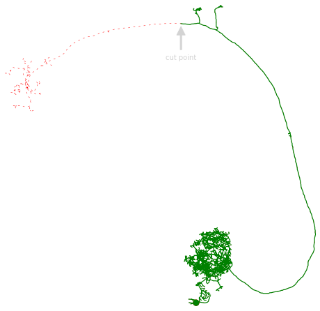
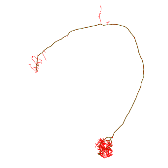
Instead of cutting a neuron in two, we can also just prune bits off:
n_pruned = n.prune_distal_to(cut_node_id, inplace=False)

cut_coords = n.nodes.set_index('node_id').loc[cut_node_id, ['x', 'z']].values

# Plot original neuron in red and with dotted line
fig, ax = n.plot2d(color='red', method='2d', linestyle=(0, (5, 10)), view=('x', '-z'))

# Plot remaining neurites in red
fig, ax = n_pruned.plot2d(color='green', method='2d', ax=ax, view=('x', '-z'), lw=1.2)

# Annotate cut point
ax.annotate('cut point',
            xy=(cut_coords[0], -cut_coords[1]),
            color='lightgrey',
            xytext=(cut_coords[0], -cut_coords[1]-2000), va='center', ha='center',
            arrowprops=dict(shrink=0.1, width=2, color='lightgrey'),
            )

plt.show()
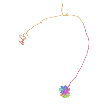
cut_skeleton() also takes multiple cut nodes, in case you want to chop your neuron into multiple pieces.
As an (extreme) example, let’s cut a neuron at every single branch point:
n = navis.example_neurons(1, kind='skeleton')

branch_points = n.nodes[n.nodes.type=='branch'].node_id.values

cut = navis.cut_skeleton(n, branch_points)
cut.head()
| type | name | id | n_nodes | n_connectors | n_branches | n_leafs | cable_length | soma | units | created_at | id | origin | |
|---|---|---|---|---|---|---|---|---|---|---|---|---|---|
| 0 | navis.TreeNeuron | DA1_lPN_R | 1734350788 | 4 | 16 | 0 | 2 | 373.565735 | None | 8 nanometer | 2022-07-27 21:19:57.584201 | 1734350788 | /Users/philipps/Google Drive/Cloudbox/Github/n... |
| 1 | navis.TreeNeuron | DA1_lPN_R | 1734350788 | 5 | 10 | 0 | 2 | 431.518494 | None | 8 nanometer | 2022-07-27 21:19:57.584201 | 1734350788 | /Users/philipps/Google Drive/Cloudbox/Github/n... |
| 2 | navis.TreeNeuron | DA1_lPN_R | 1734350788 | 6 | 12 | 0 | 2 | 388.590637 | None | 8 nanometer | 2022-07-27 21:19:57.584201 | 1734350788 | /Users/philipps/Google Drive/Cloudbox/Github/n... |
| 3 | navis.TreeNeuron | DA1_lPN_R | 1734350788 | 8 | 22 | 0 | 2 | 665.534912 | None | 8 nanometer | 2022-07-27 21:19:57.584201 | 1734350788 | /Users/philipps/Google Drive/Cloudbox/Github/n... |
| 4 | navis.TreeNeuron | DA1_lPN_R | 1734350788 | 28 | 8 | 0 | 2 | 1534.385498 | None | 8 nanometer | 2022-07-27 21:19:57.584201 | 1734350788 | /Users/philipps/Google Drive/Cloudbox/Github/n... |
# Plot neuron fragments
fig, ax = navis.plot2d(cut, linewidth=1.5)

# Rotate to front view
ax.azim, ax.elev = -90, -90
ax.dist = 6

plt.show()
Let’s try something more sophisticated: pruning by Strahler index.
# Load a fresh skeleton
n = navis.example_neurons(1, kind='skeleton')

# Reroot to soma
n = n.reroot(n.soma)

# This will prune off terminal branches (the lowest two Strahler indices)
n_pruned = n.prune_by_strahler(to_prune = [1, 2], inplace=False)

# Plot original neurons in red
fig, ax = n.plot2d(color='red')

# Plot remaining neurites in green
fig, ax = n_pruned.plot2d(color='green', ax=ax, linewidth=1)

# Rotate to front view
ax.azim, ax.elev = -90, -90
ax.dist = 6

plt.show()
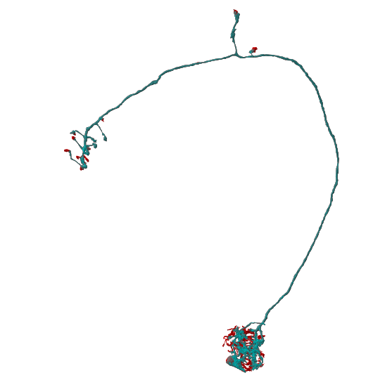
We can also turn this around and remove only the higher order branches. Let’s use this example to show that we can also do this with MeshNeurons:
# Load an example mesh neuron
m = navis.example_neurons(1, kind='mesh')

# This will prune to the just terminal branches
m_pruned = navis.prune_by_strahler(m, to_prune=range(3, 100), inplace=False)

# Plot original neuron in cyan
fig, ax = m.plot2d(color='cyan', figsize=(10, 10))

# Plot remaining neurites red
fig, ax = m_pruned.plot2d(color='red', ax=ax)

# Rotate to front view
ax.azim, ax.elev = -90, -90
ax.dist = 6

plt.show()
Alternatively, we can prune terminal branches based on size:
# This will prune all branches smaller than 10 microns
m_pruned = navis.prune_twigs(m, size='10 microns', inplace=False)

# Plot original neuron in red
fig, ax = m.plot2d(color='red', figsize=(10, 10))

# Plot remaining neurites in cyan
fig, ax = m_pruned.plot2d(color='cyan', ax=ax, linewidth=.75, alpha=.5)

# Rotate to front view
ax.azim, ax.elev = -90, -90
ax.dist = 6

plt.show()
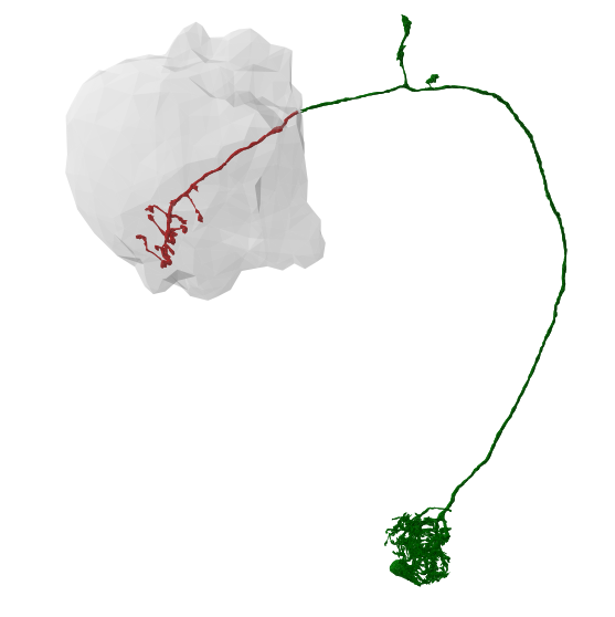
Intersecting with Volumes
We can also intersect neurons with navis.Volume (and trimesh.Trimesh for that matter).
# Load an example navis.Volume
lh = navis.example_volume('LH')

# Prune by volume
m_lh = navis.in_volume(m, lh, inplace=False)
m_outside_lh = navis.in_volume(m, lh, mode='OUT', inplace=False)
And plot!
# Plot pruned branchs neuron in green
fig, ax = navis.plot2d([m_lh, m_outside_lh, lh], color=['red', 'green'], figsize=(10, 10))

# Rotate to front view
ax.azim, ax.elev = -90, -90
ax.dist = 6

plt.show()
Does this work with all neuron types? There is no simple answer unfortunately. In theory, anything that works on skeletons should also work on meshes, and vice versa. However, Dotprops and VoxelNeuron are so fundamentally different that certain operations just don’t make sense. For example we can’t cut them but we can subset them to a given volume. Check out the API docs for an overview of what works with which neuron type.
Note that navis.in_volume() also works with arbitrary spatial data (i.e. (N, 3) arrays of x/y/z locations):
# Get the connectors for one of our above skeletons
cn = sk.connectors

# Add a column that tells us which connectors are in the LH volume
cn['in_lh'] = navis.in_volume(cn[['x', 'y', 'z']].values, lh)
cn.head()
| connector_id | node_id | type | x | y | z | roi | confidence | in_lh | |
|---|---|---|---|---|---|---|---|---|---|
| 0 | 0 | 1436 | pre | 6444 | 21608 | 14516 | LH(R) | 0.959 | True |
| 1 | 1 | 1436 | pre | 6457 | 21634 | 14474 | LH(R) | 0.997 | True |
| 2 | 2 | 2638 | pre | 4728 | 23538 | 14179 | LH(R) | 0.886 | True |
| 3 | 3 | 1441 | pre | 5296 | 22059 | 16048 | LH(R) | 0.967 | True |
| 4 | 4 | 1872 | pre | 4838 | 23114 | 15146 | LH(R) | 0.990 | True |
# Count the number of connectors (pre and post) in- and outside the LH:
cn.groupby(['type', 'in_lh']).size()
type  in_lh
post  False    1978
      True      106
pre   False     325
      True      296
dtype: int64
About half the presynapses are in the LH (most of the rest will be in the MB calyx). The large majority of postsynapses are outside the LH in the antennal lobe where this neuron has its dendrites.
That’s it for now! Please see the NBLAST tutorial for morphological comparisons using NBLAST and the API for a full list of morphology-related functions.